Quick Start

This quick start tutorial will demonstrate the basic usage of dnamite. For more detailed usage see the user guides.

import numpy as np
import pandas as pd
import seaborn as sns
sns.set_theme()
from sklearn.model_selection import train_test_split

Why Use dnamite?

Given a set of \(p\) features \(X\), dnamite trains additive models with the form \(f(X) = \sum_j f_j (X_j)\). Such additive models maintain similar structure to linear models but allow each feature function (also known as shape function) \(f_j\) to be nonlinear thus improving predictive accuracy. By maintaining additive structure, a trained dnamite model can directly describe its predictions via shape functions, and can summarize the importance of each feature via feature importance scores. Therefore, dnamite is suitable when both accuracy and interpretability are important. For more details see the Why dnamite User Guide.

Regression

We’ll start by importing some packages and reading in the California Housing dataset, a standard regression dataset. The task is to predict the median house value for a given district in California. No data preprocessing is requires as dnamite can handle missing values and categorical features natively.

from sklearn.datasets import fetch_california_housing
data = fetch_california_housing(as_frame=True)
X, y = data["data"], data["target"]
X_train, X_test, y_train, y_test = train_test_split(X, y, test_size=0.2, random_state=10)

To fit a dnamite model, we use DNAMiteRegressor. Binary classification is very similar but with DNAMiteBinaryClassifier. The only required input parameter is n_features, which should be set to the number of features in our training dataset. We pass two additional optional parameters: 1) device, which allows for GPU training if available, and 2) num_pairs, which asks the model to include a set number of pairwise interaction.

from dnamite.models import DNAMiteRegressor

model = DNAMiteRegressor()
model.fit(X_train, y_train)

DNAMiteRegressor(random_state=672)

In a Jupyter environment, please rerun this cell to show the HTML representation or trust the notebook.
On GitHub, the HTML representation is unable to render, please try loading this page with nbviewer.org.

Let’s first check that our fitted model has reasonable predictive accuracy by comparing to a black-box ML model from scikit-learn.

preds = model.predict(X_test)
print(f"DNAMite RMSE: {np.sqrt(np.mean((preds - y_test)**2))}")

# Compare to an sklearn model
from sklearn.ensemble import HistGradientBoostingRegressor
gbr = HistGradientBoostingRegressor()
gbr.fit(X_train, y_train)
preds = gbr.predict(X_test)
print(f"HistGBR RMSE: {np.sqrt(np.mean((preds - y_test)**2))}")

DNAMite RMSE: 0.578846313081703
HistGBR RMSE: 0.474020920829243

We can now start interpreting our model. First we can look at the top feature importances from the model.

model.plot_feature_importances()

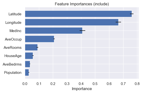
Latitude and longitude are important terms in the model, which makes sense for predicting house prices in a state like California. The median income of the district is also an important predictor.

Now we can plot shape functions for some of the more important terms in the model. Since the trained model is additive, these plots directly describe how each feature contributes to the final prediction.

model.plot_shape_function(["MedInc", "AveOccup", "AveRooms"])

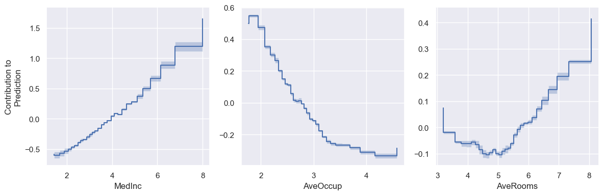
As expected, median income and average number of rooms are positively correlated with house price. Meanwhile, it’s perhaps less expected that average number of occupants is negatively correlated with house price.

We can also add feature interactions to dnamite models. Setting the pairs_list parameter in the fit functions sets a fixed list of interactions to add to the model.

model = DNAMiteRegressor()
model.fit(X_train, y_train, pairs_list=[["Latitude", "Longitude"]])

DNAMiteRegressor(random_state=344)

In a Jupyter environment, please rerun this cell to show the HTML representation or trust the notebook.
On GitHub, the HTML representation is unable to render, please try loading this page with nbviewer.org.

We can then visualize the fitted interaction using a heatmap.

model.plot_pair_shape_function("Latitude", "Longitude")

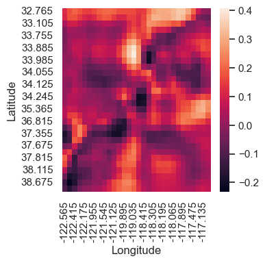
The latitude/latitude interaction plot shows a few spots of lower and higher median house values. For example, the lightest spot around (34, -118.5) corresponds to Los Angeles.